

Natural Gas is a highly volatile commodity whose price is impacted by various supply and demand factors.
The supply-side factors include:
Natural gas production
Natural gas storage
Natural gas imports and exports
The demand-side factors include:
Variations in winter and summer weather
Economic growth
Availability and prices of other fuels
On the demand side, one of the most significant factors influencing short-term fluctuations in price is temperature variations which heavily impact the demand for natural gas due to the use of natural gas in heating and cooling in summer and winter months.
This implies that temperature has a causal effect on the demand for natural gas and thus indirectly its price.
To test this theory we firstly need to obtain the relevant price and temperature data this can be done in Python using the yfinance API to retrieve natural gas prices and the meteostat API to retrieve historical temperature data.
import yfinance as yf
import pandas as pd
import matplotlib.pyplot as plt
import datetime as dt
from meteostat import Point, Daily
#Get Nat Gas 2015 price
NG = yf.Ticker("NG=F").history(period="108mo")['Close']
#Set start and end date for temperature data
start = dt.datetime(2015, 1, 1)
end = dt.datetime(2024, 1, 1)
# Create Point for London, UK
location = Point(51.5072, -0.1276, 70)
# Get daily data since 2015
data = Daily(location, start, end)
data = data.fetch()
# Plot line chart including average, minimum and maximum temperature
data.plot(y=['tavg', 'tmin', 'tmax'])
plt.show()
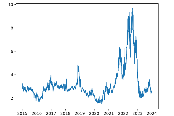
#Plot Natural Gas Prices
plt.plot(NG)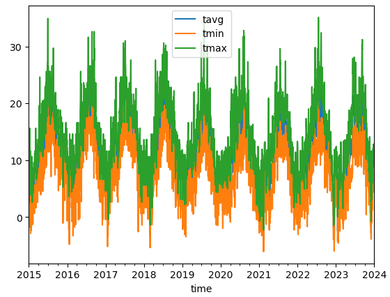
For simplicity, we will be using London as our representative temperature in this model however a useful and accurate model should consider the use of population-weighted average temperatures across Europe and North America in cities where natural gas is used.
To convert the temperature data into a useful measure we will get the absolute difference of every temperature point from 20 degrees Celsius shown by the formula below.
This formula allows us to see when the temperature deviates from what is considered a comfortable temperature (20 degrees) to either the upside or downside which is theoretically indicative of an increase in demand for natural gas.
We can then run a polynomial regression to the 5th degree where x = ABSDiff to use the temperature values to explain natural gas price as shown below.
After running this regression model we get an R-squared value of 0.0147 meaning we can only explain 1.47% of the variation in natural gas prices over the 9-year period with this regression model.
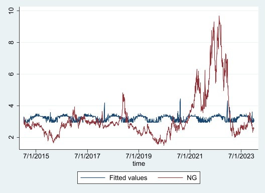
This model on its own for predicting natural gas prices is of little use however it does help to prove the impacts of seasonal trends on prices and can help to serve as a foundation for a more intricate model including further supply and demand factors.